Performance analysis of TSCH and Orchestra
Introduction
This project is a benchmark of the performance of TSCH and Orchestra compared to CSMA and 6TiSCH with IoTlab environment.
Project structure
Project presentation
The aim of this project is to compare the performance of the TSCH protocol with CSMA in non-beacon mode, and to compare the performance of the Orchestra scheduler with Contiki's default scheduler, 6TiSCH, in an IoT network with several configurations. Indeed, Time Slotted Channel Hopping (TSCH) is a MAC protocol that reduces energy consumption and increases network reliability, and Orchestra is a standalone scheduling solution for TSCH that, with the use of RPL, improves the latency-energy balance and reduces network packet loss.
To carry out this project, we used the IoTLab test platform, which enables experiments to be deployed on real IoT nodes via an API or command line via an SSH connection. In this way, we created experiments containing different nodes using TSCH and Orchestra. We set up groups of experiments targeting the analysis of a particular metric, where each experiment contained different configurations. As a result, we were able to obtain results that we could analyze.
Node type and firmware
For this project, we used two types of node: coordinator and sender. Nodes of the coordinator type are intended to synchronize nodes, receiving data frames from the sender and sending a data frame back to the coordinator. Sender nodes send data frames to the coordinator. Each type of node has its own firmware written in C: coordinator.c and sender.c. A Makefile supplied with the firmware is used to build executables (in .iotlab) adapted to the platform's IoT nodes. It lets you choose the MAC protocol to be implemented and its orchestrator. A configuration file named project-conf.h is used to modify the TSCH and Orchestra configurations. For each experiment, we decided to implement one coordinator and several sender in order to observe each metric on that particular coordinator. The main reason for this choice is that we believe that if several coordinators are implemented, the load distributed between them will not necessarily be the same from one experiment to another, and so will skew the results.
Automation scripts
To automate the deployment of experiments, we have created scripts that enable us to deploy experiments on the IoTLab platform, monitor node energy consumption, retrieve network traffic and analyze it.
Bash script:
- submit.sh: this script is used to deploy an experiment on the IoTLab platform. It takes as parameters the name of the experiment, the duration of the experiment, the number of nodes, the site on which the experiment is to be deployed and the type of MAC protocol used (CSMA or TSCH). It creates a JSON file containing the experiment information and sends it to the IoTLab API. It then waits for the experiment to be deployed and displays the experiment ID.
- check_free_node.sh: this script checks the number of nodes available on a site. It takes the site name as parameter. It displays the nodes available on the site.
- stop.sh: this script is used to stop an experiment. It takes the ID of the experiment to be stopped as a parameter. It sends a request to the IoTLab API to stop the experiment.
- monitor.sh: this script is used to launch an experiment with a metric to be observed (power consumption or radio activity). It takes as parameters the name of the experiment, the duration of the experiment, the number of nodes, the metric to be observed and the type of MAC protocol used (CSMA or TSCH). The results of the experiment can then be displayed using the monitor.py script. This script cannot select the experiment site, as via an SSH connection it is only possible to retrieve power and radio activity information from the site linked to your IoTLab account.
- netcat.sh: this script is used to retrieve network traffic. It takes as parameters the name of the experiment, the duration of the experiment, the number of nodes, the site on which the experiment is to be deployed and the type of MAC protocol used (CSMA or TSCH). It retrieves network traffic data from each node until the end of the experiment. The data is written to text files saved in a directory named netcat.
- monitor_netcat.sh: this script launches an experiment with a metric to be observed (power consumption or radio activity) and retrieves the network traffic. It takes as parameters the name of the experiment, the duration of the experiment, the number of nodes, the metric to be observed and the type of MAC protocol used (CSMA or TSCH). It is based on monitor.sh and netcat.sh.
- sniffer.sh: this script is used to save global network traffic via the serial_aggregator command. It takes the same parameters as the netcat.sh script. The results are saved in text files in the sniffer folder.
It is important to note that each script is independent of the other, so submit.sh is not required to run netcat.sh or monitor.sh.
Python script:
- monitor.py: this script allows you to observe the power consumption and/or radio activity of nodes. It takes as parameters the ID of the experiment, the duration, whether power consumption or radio activity is to be observed, the type of node to be observed (coordinator or sender) and the desired result. If the argument is left blank, a value is displayed in the terminal (average power consumed or duty cycle of each channel), otherwise it displays graphs directly (plot).
- netcat.py: this script allows you to observe network connection times, the percentage of successful data transmission (PDR) and the duration of a ping as a function of the number of nodes. It produces three graphs, displaying results for CSMA and TSCH. It takes no parameters.
Each python script needs to be run in the current Git directory.
Description of the scenarios studied
For the chosen scenarios, we modified several aspects of the firmware configuration (MAC protocol, orchestrator etc...) and carried out several experiments with different characteristics.
Firmware configuration
The aim of this project is to analyze the performance of TSCH and Orchestra, so we decided to adopt one scenario where they would be used and another where they would not. We have therefore divided our configuration scenarios into three main cases:
| CSMA | TSCH | Orchestra | |
|---|---|---|---|
| Case 1 | ✓ | ✕ | ✕ |
| Case 2 | ✕ | ✓ | ✕ |
| Case 3 | ✕ | ✓ | ✓ |
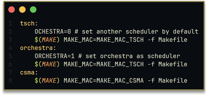
To facilitate the transition from one case to another, we've added 3 rules to the Makefile. The first is to compile files with CSMA, the second with TSCH and a default orchestrator provided by Contiki: 6TiSCH, and the last allows TSCH to be compiled with Orchestra as orchestrator.
Experimental setup
To make sense of the different firmware configurations, we decided to run several experiments on each case. Basically, we used a similar format for each case, as follows:
- 1 coordinator / 1 sender
- 1 coordinator / 3 sender
- 1 coordinator / 9 sender
- 1 coordinator / 24 sender
We sometimes carried out an additional experiment with 49 sender to try and observe the accentuation of certain metrics. We then decided to adapt the duration of the experiments according to the metrics we were measuring. We were able to carry out experiments lasting 2 and 10 minutes, as well as those lasting an hour.
Metrics used
First, we observed the power consumption and radio activity of the coordinator or a sender. To do this, we used a graph showing the evolution of power consumption over time, a graph showing radio activity over time, as well as the average power consumed and the average period between each radio wave received. Secondly, we analyzed network traffic. We evaluated the network connection time for all nodes, the percentage of successful data transmission applications for all nodes, and the average ping time between two nodes.
Results
Observation of power evolution
We carried out one experiment per case (n°1, n°2, n°3), observing the evolution of the power consumed by the coordinator (below left) and by the sender (below right). We ran each case for 120 minutes, with one coordinator and one sender.
Case 1 : CSMA
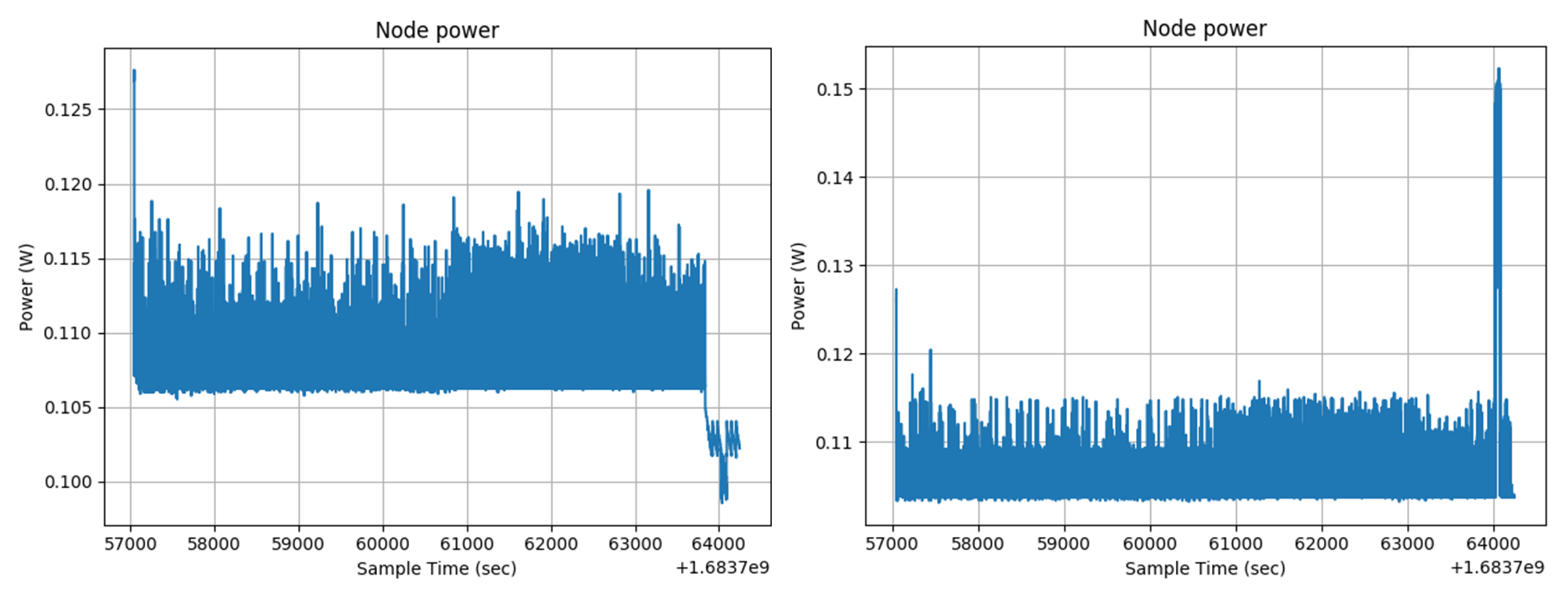
We measured an average power consumption for each node of :
- coordinator : 31.76 mW
- sender: 31.85 mW
In this case, 49 messages were transmitted correctly, representing 0.65 mW per message.
Case 2 : TSCH
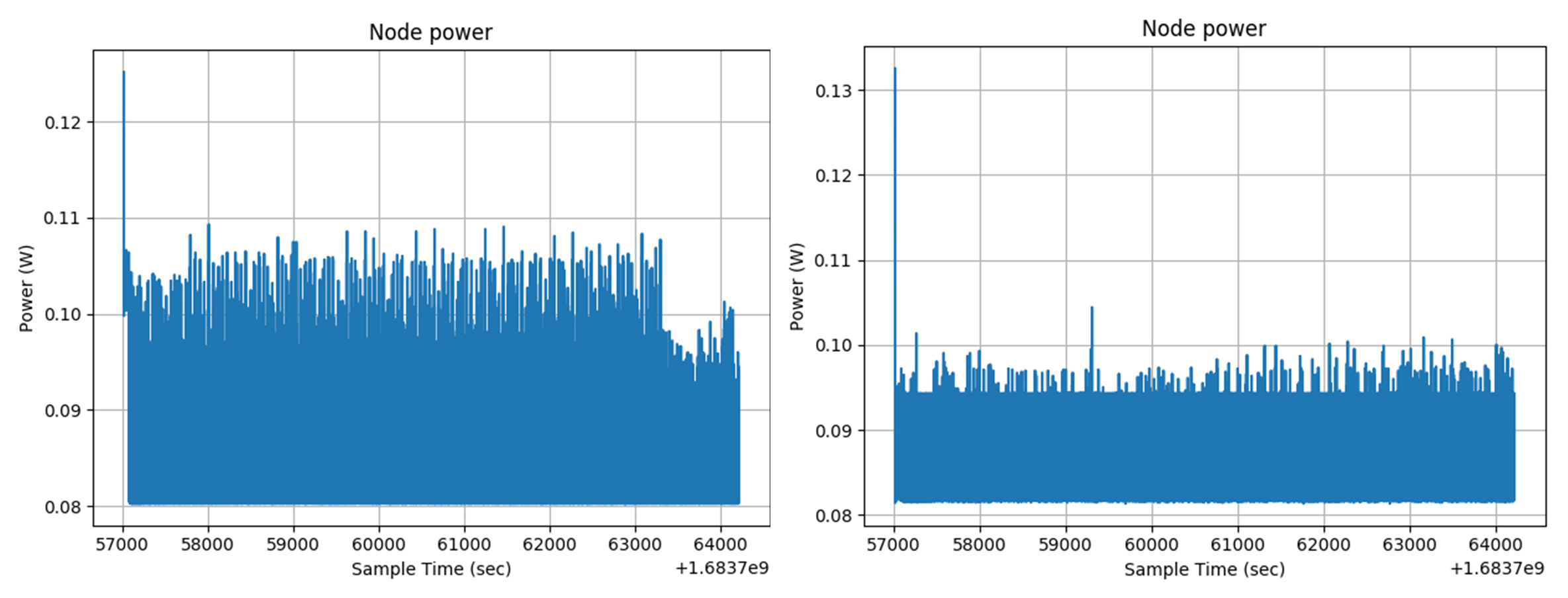
We measured an average power consumption for each node of :
- coordinator: 26.93 mW
- sender: 27.21 mW
In this case, 48 messages were transmitted correctly, representing 0.57 mW per message.
Case 3 : Orchestra
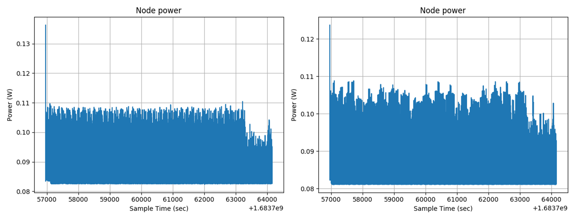
We measured an average power consumption for each node of :
- coordinator: 26.96 mW
- sender: 26.84 mW
In this case, 36 messages were transmitted correctly, representing 0.75 mW per message.
We ran this experiment several times to check that the orders of magnitude of power consumption were respected for each experiment.
Observing radio activity
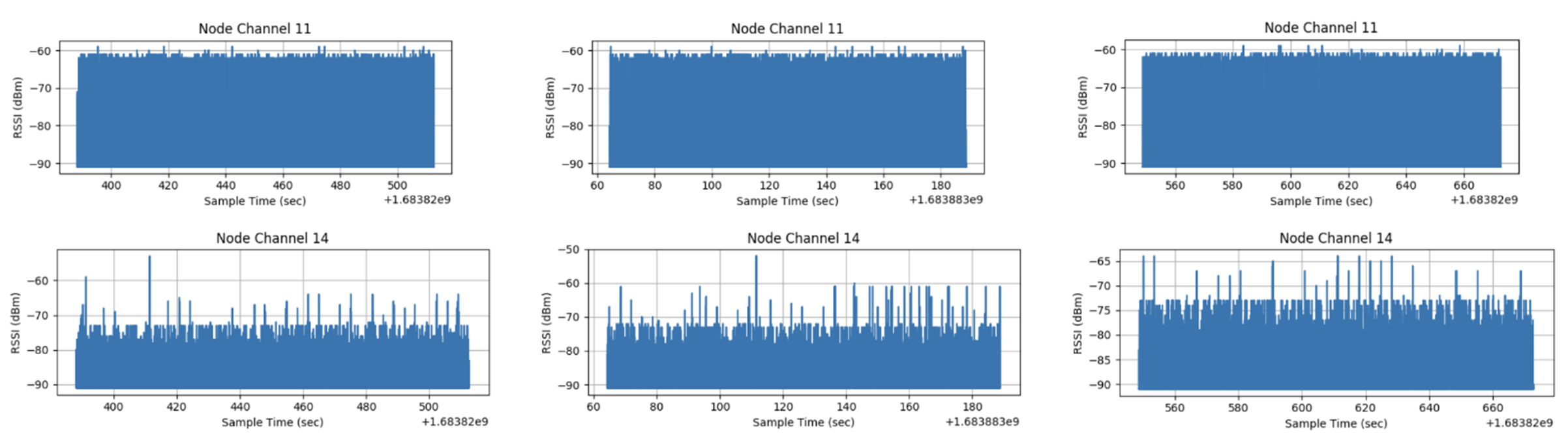
We ran several experiments per case (n°1, n°2, n°3), observing radio activity per channel (11 and 14). In all, we ran 4 experiments per case for 2 minutes at 2, 4, 10 and 25 knots. The graphs for CSMA are below on the left, those for orchestra below in the middle and those for TSCH below on the right.
Experiment 1 : 2 nodes
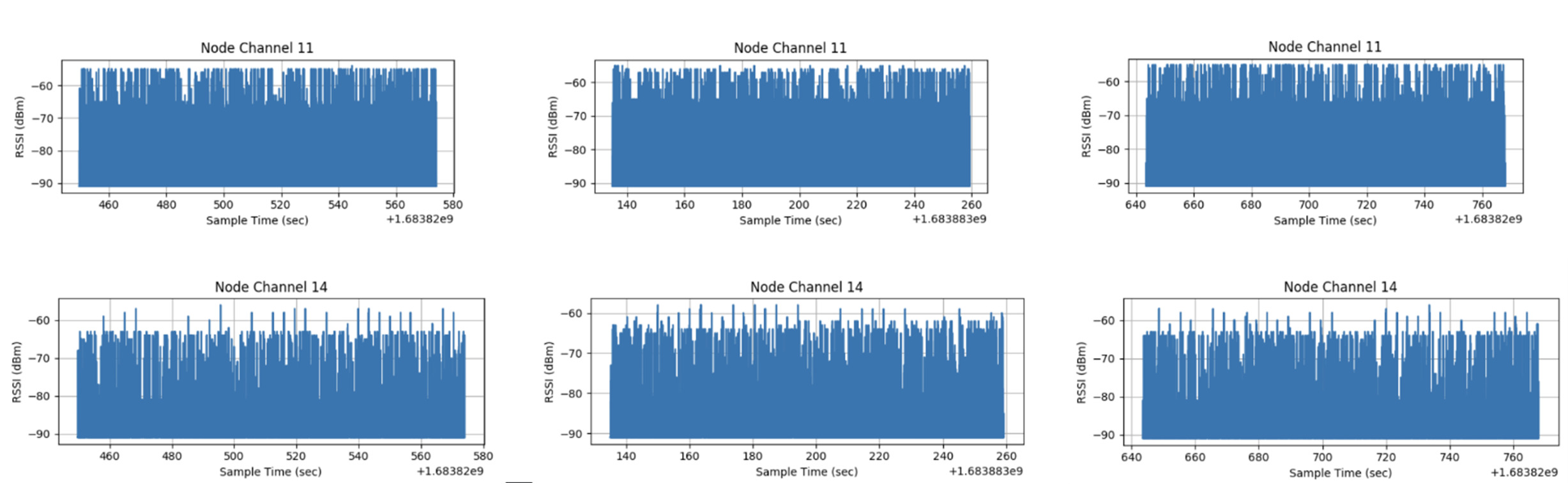
Experiment 2 : 4 nodes
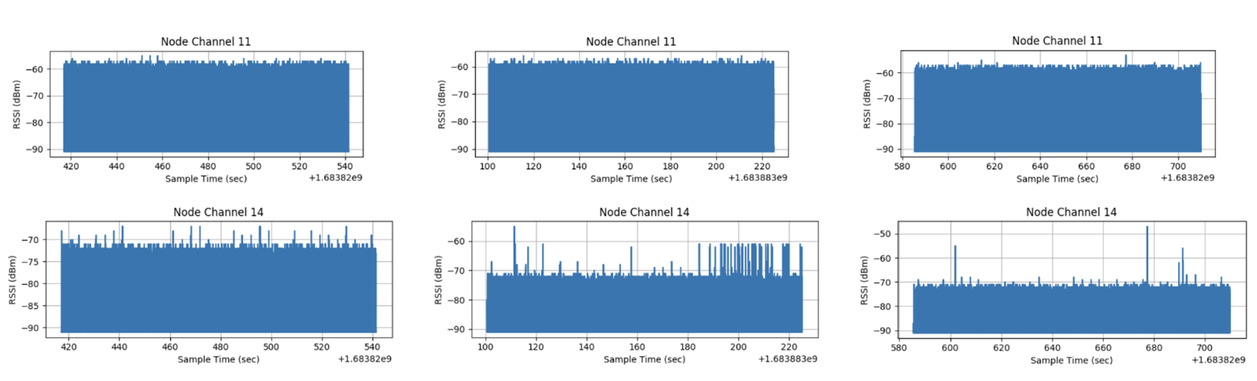
Experiment 3 : 10 nodes
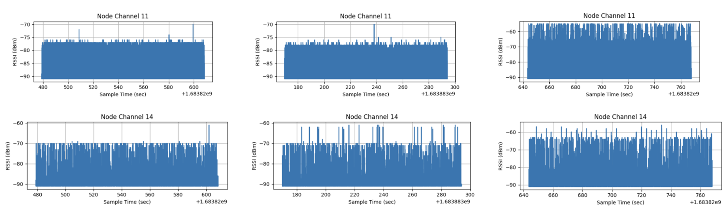
Experiment 4 : 25 nodes
Observation of times and percentage of success
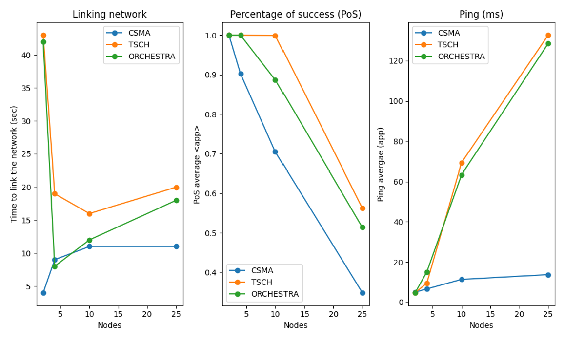
We carried out several case experiments (n°1, n°2, n°3), in which we observed network connection time (RPL initialization time), the percentage of successful application data transmission and the application communication delay between coordinator and sender (ping). We plotted graphs showing the evolution of these characteristics according to the number of nodes present (2, 4, 10 and 25 nodes).
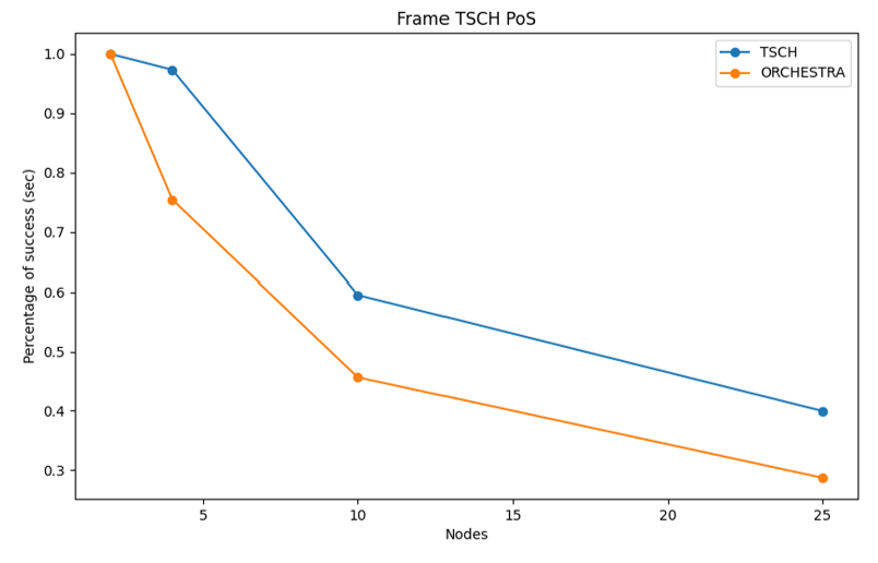
Observation of the percentage of success depending on the orchestrator
We carried out an experiment in which we observed the percentage of successful data transmission between two orchestrators: Contiki's default orchestrator, 6TiSCH, and Orchestra.
Analysis of results
Analysis of power consumption
We can see that these graphs show similar trends. For both node types, we observe a power peak at the beginning of the experiment, which represents the initialization phase. Power then stabilizes between a higher value (peak) and a lower value (valley), showing the alternation between awake (listening or transmitting) and asleep modes. What's more, we can see from the average power consumption that TSCH consumes less than CSMA, and that Orchestra makes no major change to energy consumption compared with 6TiSCH.
Analysis of radio activity
We can observe that the graphs for channel 11, whatever the experiment and the case, show a similar evolution, only the average RSSI changes according to the experiment. It is the same in each case and experiment, except for the 25-knot experiment, where CSMA and TSCH + Orchestra show a decrease, unlike TSCH + 6TiSCH. This is normal, since there are more nodes and therefore more radio activity, which in turn reduces signal strength. However, for TSCH + 6TiSCH, we can assume that it's due to 6TiSCH that the average RSSI remains so high. We can see that the graphs for channel 14 show similar trends in each case, with fewer and fewer isolated peaks as the number of nodes increases. As for the average RSSI, it is equivalent in each case according to experience. We can see that TSCH + Orchestra shows more disparities than the other cases, which may be due to poor configuration on our part or the influence of other experiments on radio activity in channel 14. In addition, we have calculated the duty cycle for each channel, but we obtain values such as 50.00 ± 0.05%. It is therefore difficult to draw any conclusions, especially as there is no proportionality according to the protocols used or the number of nodes.
Analysis of times and percentage of success
In terms of network connection time, we can see that TSCH and TSCH with Orchestra have a significant network connection time for a sender and a coordinator, but that this becomes acceptable for more nodes. We note that CSMA is the fastest to converge and Orchestra is slightly faster than 6TiSCH. The convergence time takes into account the convergence of RPL and also the planning time of TSCH (hence the discrepancy measured). For the percentage of success, they are all error-free with a single sender, but they all decrease significantly as a function of the number of nodes. However, TSCH, and to a lesser extent Orchestra, maintain a 100% success rate even beyond 1 sender (> 4 for TSCH + Orchestra and > 10 for TSCH + 6TiSCH). We can assume that TSCH, thanks in particular to the orchestrator, maintains a 100% success rate up to a certain number of nodes, but that beyond this number, the load becomes too great for the coordinator. For ping, CSMA keeps ping almost constant, whereas TSCH and Orchestra's ping increases greatly with the number of nodes. This is undoubtedly due to the fact that TSCH is a heavier protocol for the coordinator, so the more nodes there are, the longer it takes to reply to the sender, whereas CSMA is much simpler.
We can therefore deduce that TSCH improves reliability at the cost of speed, while CSMA improves speed at the cost of reliability.
Percentage success analysis by scheduler
We can observe that the percentage of success at MAC level is to the advantage of TSCH (with 6tisch), yet Orchestra promises an improvement in speed. However, Orchestra contains a large number of configuration parameters, and we have chosen to use the default configuration, which may not be the most appropriate in our case. For example, we could have adapted the slotframe size. What's more, we've found that Orchestra outperforms 6TiSCH for experiments lasting longer than 10 minutes (over 2 hours). For example, we carried out two 2-hour experiments with 4 nodes, one with TSCH and 6TiSCH and the other with TSCH and Orchestra. We obtained the following results:
| TSCH + 6TiSCH | TSCH + Orchestra | |
|---|---|---|
| Application success rate | 99.27% | 99.46% |
| Application communication time | 20.8s | 11.0s |
| Success rate according to TSCH logs | 70.8% | 98.1% |
Conclusion
We have therefore been able to observe the promises made by TSCH with regard to CSMA in non-beacon mode, i.e. to reduce energy consumption and increase reliability by reducing packet loss. As far as Orchestra is concerned, we have not been able to observe the promises made to 6TiSCH. However, in a second phase, we were able to observe them in a 2-hour experiment, where Orchestra outperformed 6TiSCH while consuming similar amounts of energy. We therefore conclude that to achieve better analysis and comparison between schedulers, it is necessary to carry out long experiments.